Welcome

This mini-course will be structured around four themes.

1) Establishing good workflow habits

2) Learning how to R

3) Performing data analysis

4) Graphing

Every time you are working in R, it should be in a project

Projects are R's way of helping you keep all of your files in one place. It may seem like an unnecessary step, but trust me that it will make your life so much easier to get in the habit of working in R projects.

What is an R script?

R Scripts are where you keep all of your important code. They are also where you explain your workings and the code to yourself so that you can remember to do the same thing again later.

To make your life as easy as possible, you should generally have R Scripts that look like this:

#12 March 2020: This R Script is an example of what a good R script looks like
##
1+1 #I can't remember what 1+1 is- this way, R will tell me!

## [1] 2

Another example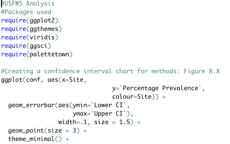

How to use R studio

R Studio has a lot of in-built tools that help with effective coding.

For example, R will automatically close parantheses and quotation marks for you; however, you need to be careful that this doesn't cause mistakes.

R Studio will also show you when you make a mistake in your R Script, through red lines underlining code and a red "X"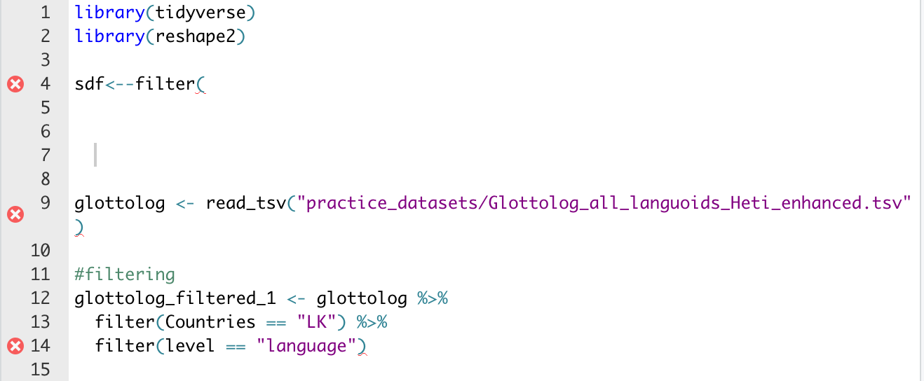

You can see here where R is telling you that your code is faulty.

You can also see that R Studio will color code differently according to its attribute: a different color for non-code "objects", for comments, and for "significant" commands like telling R which library to use.

Error Codes

What do to do when you get an error code

Read the code. This seems self-explanatory but it is where you can gain some understanding of what went wrong.

As an example, what happens if you type "b" and press enter?

You should see "Error: object 'b' not found"

This message has three parts

1) It tells us that it is an error

2) The location of the error, which is object "b"

3) The problem this mistake caused: there is no object b, because I haven't created it!

Sometimes errors are difficult to understand

If you can't understand the error message immediately, then you have several options:

1) Check out the help file for the function/command you are using, if applicable

2) Google it!

3) Ask for help from Stack Overflow (bearing in mind that it can be challenging) or from R-Ladies (if you are a woman)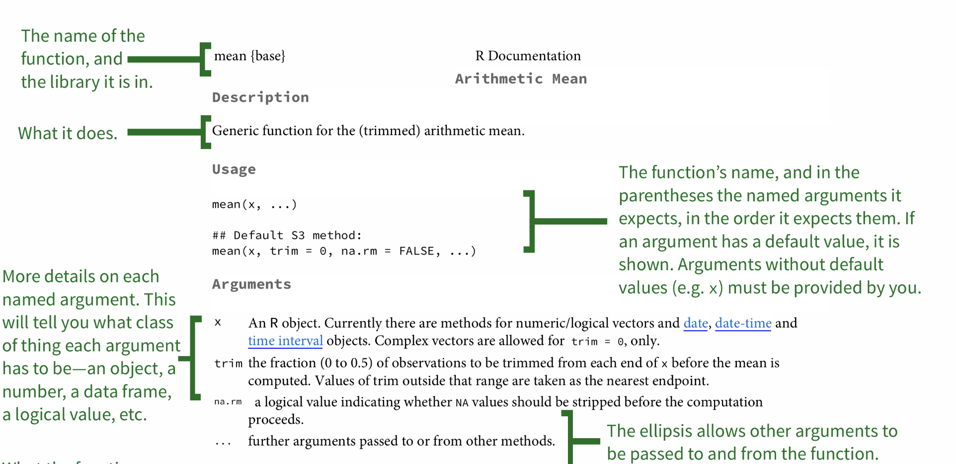

Moving on... What are packages?

Packages are extra functions or groups of functions that other people have created to help make everyone's life easier. They can be downloaded from CRAN (the R repository) or from GitHub.

This is very easy to do. Go ahead and run the following command:

#install.packages("devtools")

You now have the package "devtools" which will allow you to call packages from GitHub. Sometimes packages live on GitHub for somewhat mysterious reasons that I won't get into here.

Let's install a package from GitHub. Go ahead and run the following code:

#I have hashed it out so that I don't install it
#devtools::install_github("hadley/emo", force = "true")

You now have the "emoji" package downloaded! Try the following:

emo::ji("party")

## 🎉

Getting Data into R

Go to the following site:

https://vincentarelbundock.github.io/Rdatasets/datasets.html

and download the dataset “survival”. We will read this into R using the following command:

Hanoi<-read.csv("survival.csv")

When you read this into R, you should see the following: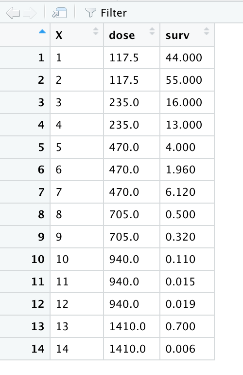

And over in your top right pane, you will see "Hanoi" listed. It tells you how many observations there are (your n) and how many variables you have.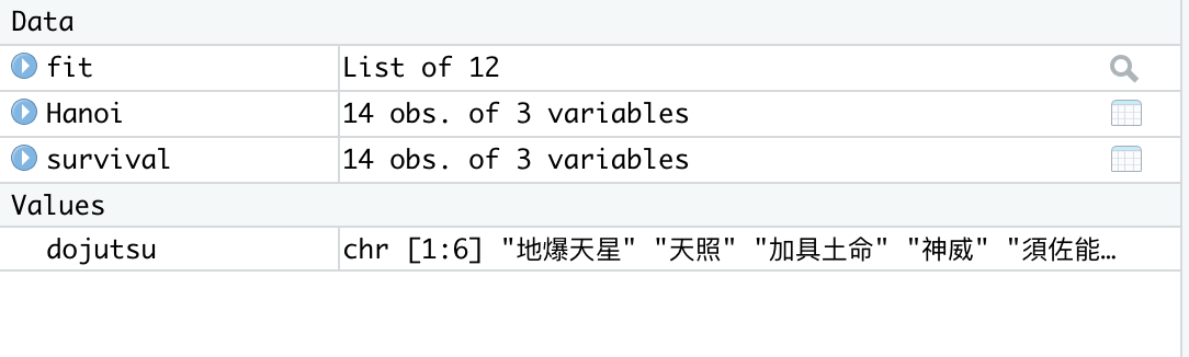

As you can see, we use the arrow to assign our dataset to a name. Therefore,when you type "Hanoi" it will show you the dataset that you have loaded into R.

However, R Studio makes things very simple by cutting out this extra step. If you look at R Studio, you’ll note that in the top right corner there’s a box that has the tab “Environment”.

You’ll see that there’s a button that says “Import dataset”. You can use this button to quickly import any dataset you desire. Try it now with the "survival" dataset you just imported into R as “Hanoi”.

A quick, basic lesson

Before we go any further, I must stress that R is very, very particular. If a command goes wrong, it is 99%¹ probable that you did not write the name of the dataset/vector/variable properly, OR that you did not put a parentheses or a comma, or some other form of punctuation where there should be one. The beauty of R studio is that it’s very good at putting parentheses in the right places, but errors still do occur.

[1] Accurate math

R is quite simply, an entirely new language. That being said, it operates in an intuitive manner. For instance, try the command we had previously in our R Script:

1+1

If you press enter, you'll see that it executes the code and gives you the answer, which is

## [1] 2

Of course, we all know what 1 + 1 is (but imagine if we didn’t!).

Assigning equations to vectors

Now, what if we wanted to assign the value of the equation 1+1 to an object in R?

a <- 1+1
a

## [1] 2

You can see that the value of this equation is stored in the object of a. Now, perhaps you can begin to see what kinds of things you can do with this object, e.g.

Using R for data analysis

"Statistics [and data analysis] is a problem-solving and decision-making process that is fundamental to scientific inquiry and essential for making sound decisions."

Taking a look at our dataset

Before starting analysis on a dataset, you need to familiarize yourself with the data. This can be done in R very easily. One command that's useful is the following, on our "Hanoi" dataset:

head(Hanoi)

##   X  dose  surv
## 1 1 117.5 44.00
## 2 2 117.5 55.00
## 3 3 235.0 16.00
## 4 4 235.0 13.00
## 5 5 470.0  4.00
## 6 6 470.0  1.96

As you can see, this shows you the top of the dataset (the "head", if you will), which is helpful if one wants to get a quick snapshot of the dataset.

The next command is:

names(Hanoi)

## [1] "X"    "dose" "surv"

Our variables here are "dose" and "survival". To give you some context, this dataset is about the survival of rats after being given radiation doses. "surv" is the survival rate of the batches expressed as a percentage, while "dose" is the dose of radiation administered (rads).

Now, it doesn't seem to make sense for our dataset to be called "Hanoi". How do you think we would go about renaming it?

survival <- Hanoi

Now, you should see in your top right pane, under "Environment", the dataset survival, which is exactly the same as the Hanoi dataset.

Summary statistics in R

This is very easy to do in R. Simply type the following:

summary(survival)

##        X              dose             surv        
##  Min.   : 1.00   Min.   : 117.5   Min.   : 0.0060  
##  1st Qu.: 4.25   1st Qu.: 293.8   1st Qu.: 0.1625  
##  Median : 7.50   Median : 587.5   Median : 1.3300  
##  Mean   : 7.50   Mean   : 654.6   Mean   :10.1250  
##  3rd Qu.:10.75   3rd Qu.: 940.0   3rd Qu.:11.2800  
##  Max.   :14.00   Max.   :1410.0   Max.   :55.0000

As you can see, this command gives you a nice little snapshot of the data, with means and medians. You can also find the mean for each specific variable by simply typing the following:

mean(survival$dose)

## [1] 654.6429

As you see, this mean is the same as the mean we see in the summary statistics we did with summary(survival).

You probably noticed the use of the "$" operator. This is your way of telling R where to "look".

When you type mean(survival$dose) you are telling R "I want the mean of the variable dose in the survival dataset."

Now on your own, try finding the median of "surv"

You should have typed in the following, and gotten the following result:

median(survival$surv)

## [1] 1.33

How do you make sense of your data?

In earlier versions of this lecture, I would tell students to investigate three key assumptions (namely, normality, homogeneity of variances, and whether samples were independent).

Nowadays, I don't think those are as important. You absolutely should understand your data, but for social scientists our data is 99%¹ of the time going to be non-normal, and often with wide variances. And as social scientists, we should already know whether our data is dependent or independent.

We can easily visualize our data with a histogram, using the hist command:

hist(survival$surv)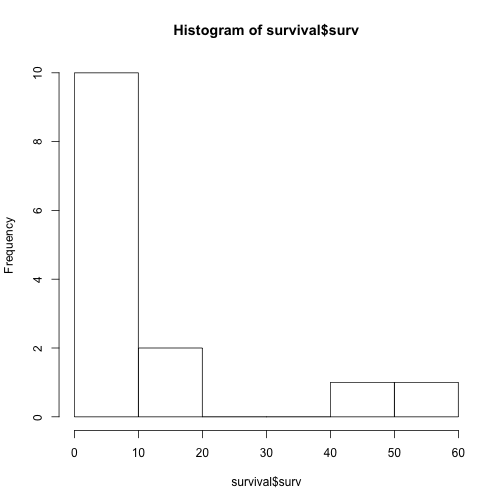

As you can see, the data really aren’t normally distributed. In fact, the data are right-skewed (i.e. a long right tail).

This tells us already that there is something going on with our data, so we should expect to see some kind of effect, depending on what we are investigating.

In the old days, we used null hypothesis significance tests (NHST)

These are now rightly criticized for obscuring the "true" effect we can see, and/or being a "lazy" way to interrogate data. Also, there are plenty of instances where it is simply unneccesary to perform NHSTs.

e.g....

Confidence intervals

These are really what you should rely on the most. A confidence interval is basically just the mean/prevalence estimate/proportion (measure we're interested in), and the margin of error (ME) multiplied by 1.96 (for 95% confidence intervals, the standard in social science).

There are plenty of ways to perform confidence intervals in R, although they all are found in packages.

For example, let's say that we want to find the confidence interval for mean survival rate.

We will install the package gmodels, and perform the following code:

We can double check this against the mean of survival, which if you'll remember is found by running:

mean(survival$surv)

## [1] 10.125

What this tells us is that our confidence interval of the mean is (-0.01, 10.1, 20.26): indicating that there is a huge amount of variance within this sample!

Although of course we already knew that, after seeing how skewed our distrubution was.

As always, having more data points will decrease your level of error.

GLMS

Often seen as scary and traumatic...

But in reality, they are pretty simple and even easy- especially with the power of R!

GLMs follow the basic formula of:

y ~ x

Where y is your dependent variable: e.g. use of bear bile, consumption of giraffe meat, whether they've poached in the last year, etc; and x is the independent variables, such as gender, age, education, etc

You also need to know what your distribution looks like, so that you can choose which GLM family is appropriate:

binomial: if you have a 0,1 dependent variable. For example, "yes" or "no" to using bear bile in the last year

poisson: count data, also sometimes called frequency. Used if you're exploring the number of times individuals in your sample used bear bile last year

gaussian: a "normal" distribution. If your dependent variable is something like height, you would use this family

GLM structure

With GLMs, you really need to think through what you're exploring. I have made many mistakes with this, and it has always come down to overcomplicating the model and/or not starting at the "top". It's best is to start with ALL of the variables you want to interrogate, something like:

bearbile ~ gender + age + province + education + religion

And working your way down based on what is significant.

For example, maybe in your "master model" only gender and education are significant.

You should then create a reduced model:

bearbile ~ gender + education

Which will give you more precise estimates of significance.

Interpreting R's GLM output

Let's say our GLM is mylogit <- glm(admit ~ gre + gpa + rank, data = mydata), where admit is whether a student got admitted to university (0,1), gre is their GRE score, gpa is of course their undergrad GPA, and rank is the relative prestige of the university.

Running your own GLM

Go ahead and explore the mtcars package in R. What are the variables? What do the data distributions look like? Note: "vs" means the probability of an engine being a certain type, "wt" is weight, and "disp" is "displacement".

Now create a GLM with the data. What will you be exploring? (You can create different versions if you like).

For example, you could have your model be glm1 <- glm(vs ~ wt + disp, mtcars, family = binomial).

If that was your model, you would then get the following output, when you ran summary:

glm1 <- glm(vs ~ wt + disp, mtcars, family = binomial) #making the model
summary(glm1)

## 
## Call:
## glm(formula = vs ~ wt + disp, family = binomial, data = mtcars)
## 
## Deviance Residuals: 
##      Min        1Q    Median        3Q       Max  
## -1.67506  -0.28444  -0.08401   0.57281   2.08234  
## 
## Coefficients:
##             Estimate Std. Error z value Pr(>|z|)  
## (Intercept)  1.60859    2.43903   0.660    0.510  
## wt           1.62635    1.49068   1.091    0.275  
## disp        -0.03443    0.01536  -2.241    0.025 *
## ---
## Signif. codes:  0 '***' 0.001 '**' 0.01 '*' 0.05 '.' 0.1 ' ' 1
## 
## (Dispersion parameter for binomial family taken to be 1)
## 
##     Null deviance: 43.86  on 31  degrees of freedom
## Residual deviance: 21.40  on 29  degrees of freedom
## AIC: 27.4
## 
## Number of Fisher Scoring iterations: 6

Hopefully you felt confident in interpreting that output! From this, we see that displacement predicts what type of engine a car will have, while weight does not. Specifically, higher displacement means that the probability of a car having a "v-shaped" engine is reduced.

Interaction terms

Another aspect of GLMs is "interaction terms". This is denoted by

*

e.g. gender ~ height * weight, where you are asking R to investigate the relationship of height and weight and how it predicts gender.

This is yet another example in R where the onus is on the operator ( i.e. you 👈 ) to have a good grasp of your data, as well as your end goal. What are you trying to prove? What exactly are you trying to understand?

One of the many wonderful aspects of R is that it really facilitates the kind of exploration that is necessary for understanding data and wriggling your way 🐛 towards enlightenment. It's easy to try different things and make different models- so you may as well do exactly that!

Also, there are tons of free resources for learning R! One great example is: https://learningstatisticswithr.com/book/introR.html.

Cleaning data is really important and something I STILL do in Excel... when it can be done so much more easily in R! This is a great resource for learning how to clean data, step by step: https://rladiessydney.org/courses/ryouwithme/

Visualization is a really important component of analysis and how you communicate your data to the world.

The easiest way to do this is by using ggplot2, Hadley Wickham's amazing "grammar of graphics".

Some important concepts:

1) "Data visualization is part art and part science." - Claus Wilke

2) Making a good visualization requires lots of practice and "material osmosis". Explore what other people are doing, get their code, and tinker!

3) ^ Tied with the above, have fun with it! Make a graph showing all the best Friends episodes or one-liners (as several people have done).

Types of graphs

1) Scatterplots/line charts ->

🍷

For #tidytuesday this week, I explored the sweet deal metric (points:price ratio) across all wine types by country, for the 15 countries with the most observations in the dataset. Yeah Chilean wine.

Code: https://t.co/WvPS1UtFVE pic.twitter.com/NzMv4jl7Fb

— Allison Horst (@allison_horst) May 29, 2019

Install and/or load the following packages:

library(tidyverse)   # All the fun tidy functions!
library(paletteer)

Now load the data: google "Allison Horst github tidy_tuesday_5_28_19", and a link to the data will come up

Or copy this long freaking thing out:

wine_ratings <- readr::read_csv("https://raw.githubusercontent.com/rfordatascience/tidytuesday/master/data/2019/2019-05-28/winemag-data-130k-v2.csv")

## Warning: Missing column names filled in: 'X1' [1]

## Parsed with column specification:
## cols(
##   X1 = col_double(),
##   country = col_character(),
##   description = col_character(),
##   designation = col_character(),
##   points = col_double(),
##   price = col_double(),
##   province = col_character(),
##   region_1 = col_character(),
##   region_2 = col_character(),
##   taster_name = col_character(),
##   taster_twitter_handle = col_character(),
##   title = col_character(),
##   variety = col_character(),
##   winery = col_character()
## )

Follow along with Allison's data manipulation in her github file

You should end up with this plot!

ggplot2 syntax

You start with your "foundational" code, which is where you tell ggplot:

• the dataset you're using

• what variable goes on the x axis

• what variable goes on the y axis

• what plot you want ggplot to generate

So we'll use something that isn't racist, and has the added benefit of being about penguins ❤️🐧.

Load the following code:

devtools::install_github("allisonhorst/palmerpenguins")

## Using github PAT from envvar GITHUB_PAT

## Downloading GitHub repo allisonhorst/palmerpenguins@master

##   
   checking for file ‘/private/var/folders/lw/rzb9nnl16xq73y25y8v73zfw0000gn/T/RtmpwktobE/remotescfc46620b41c/allisonhorst-palmerpenguins-f13c212/DESCRIPTION’ ...
✓  checking for file ‘/private/var/folders/lw/rzb9nnl16xq73y25y8v73zfw0000gn/T/RtmpwktobE/remotescfc46620b41c/allisonhorst-palmerpenguins-f13c212/DESCRIPTION’
## 
─  preparing ‘palmerpenguins’:
## 
   checking DESCRIPTION meta-information ...
✓  checking DESCRIPTION meta-information
## 
─  checking for LF line-endings in source and make files and shell scripts
## 
─  checking for empty or unneeded directories
##   
─  looking to see if a ‘data/datalist’ file should be added
## 
─  building ‘palmerpenguins_0.1.0.tar.gz’
## 
##

require(palmerpenguins)

## Loading required package: palmerpenguins

Let's make a plot!

First, go ahead and explore the data (remember, to load the data from a package you will type data("penguins")). Use head, str, and whatever else you want that will help you understand what's going on in this dataset.

data("penguins")
require(ggplot2)
ggplot(data = penguins, aes(x = flipper_length_mm, y = body_mass_g)) +
  geom_point(aes(color = species, shape = species))

For example, let's say you want to make the text bigger on your little graph above.

Here is what you have done:

g1 <- ggplot(data = penguins, 
                       aes(x = flipper_length_mm,
                           y = body_mass_g)) +
  geom_point(aes(color = species, 
                 shape = species))

Here is what you now will add:

ggplot(data = penguins, 
                       aes(x = flipper_length_mm,
                           y = body_mass_g)) +
  geom_point(aes(color = species, 
                 shape = species)) +
        theme(text = element_text(size=15)) +
  labs(caption = "Data by Allison Horst")

Let's move into practicing on your own. You can either stick with the penguins, or explore a dataset R already has, such as the mpg dataset.

e.g.

data(mpg)

Remember what we did earlier. How would you explore this dataset?