class: center, middle, inverse, title-slide # Using R for Data Analysis ### Elizabeth Davis ### San Diego Zoo Global ### 2019/05/08 (updated: 2020-06-30) --- <style type="text/css"> /* custom.css */ .left-code { color: #777; width: 38%; height: 92%; float: left; } .right-plot { width: 60%; float: right; padding-left: 1%; } .plot-callout { height: 225px; width: 450px; bottom: 5%; right: 5%; position: absolute; padding: 0px; z-index: 100; } .plot-callout img { width: 100%; border: 4px solid #23373B; } </style> --- # Previously, we learned the basics of R -- ## But you may have gone away still feeling like you don't know how to navigate in R "space" -- ### In these next few sections, I'll go through *how to use R scripts effectively*, *how to understand R Studio*, and *how to read an R helpfile*, which should help you with feeling more confident in using R --- # How to use R Scripts effectively -- ## Go ahead and open an R script on your R studio. It will be the icon in the top left of your console. It looks like this:  --- # R Scripts are where you keep your code that you will use for your *data analysis*. -- ## It is a record of what you have done, so that you can replicate it in the future. ¹ -- ### This is VERY important because projects sometimes take multiple days, if not weeks. .footnote[ [1] "making your analyses something that can be re-run easily as needed" ] --- # R Scripts are where you keep your code, so they are also where you should include *comments*, i.e. a way of explaining to others/your future self what you have done --- ## The most important thing is to use them as though *you may be hit on the head and lose your memory at any moment*. Be VERY clear about your process and why you are doing what you are. ---  --- #How to use R studio -- ## R Studio has a lot of in-built tools that help with effective coding. -- ## For example, R will automatically close parantheses and quotation marks for you; however, you need to be careful that this doesn't cause mistakes. -- ## R Studio will also show you when you make a mistake in your R Script, through red lines underlining code and a red "X" ---  -- ### You can see here where R is telling you that your code is faulty. -- ### You can also see that R Studio will color code differently according to its attribute: a different color for non-code "objects", for comments, and for "significant" commands like telling R which library to use. --- # Error Codes -- <img src="images/skipping-falling.gif", width = "100%"> --- class: center, middle ## "Start associating error messages with joy because it probably means you are about to learn something!" --- # What do to do when you get an error code -- ## Read the code. This seems self-explanatory but it is where you can gain some understanding of what went wrong. -- ## As an example, what happens if you type "a" and press enter? --  ---  -- ## This message has **three** parts -- ### 1) It tells us that it is an error -- ### 2) The location of the error, which is object "a" -- ### 3) The problem this mistake caused: there is no object a, because I haven't created it! --- # Sometimes errors are difficult to understand -- ## If you can't understand the error message immediately, then you have several options: -- ### 1) Check out the help file for the function/command you are using, if applicable -- ### 2) Google it! -- ### 3) Ask for help from Stack Overflow (bearing in mind that it can be challenging) or from R-Ladies (if you are a woman- sorry guys!) --- # Checking out the help file -- ## The help file can be challenging to understand, so Googling may be the easiest option for you. However, it is important to be familiar with R helpfiles. ---  ---  --- # Using R for data analysis -- ## "Statistics [and data analysis] is a problem-solving and decision-making process that is fundamental to scientific inquiry and essential for making sound decisions." -- ### Requires **critical thinking** (and practice!) --- class: center, middle ## I'm going to show you this process through working *backwards*: I'll show you results, findings, and interpretation, and from there show you how I did the data analysis. --- # Land use in the Greater Mekong Region: 2012 --- 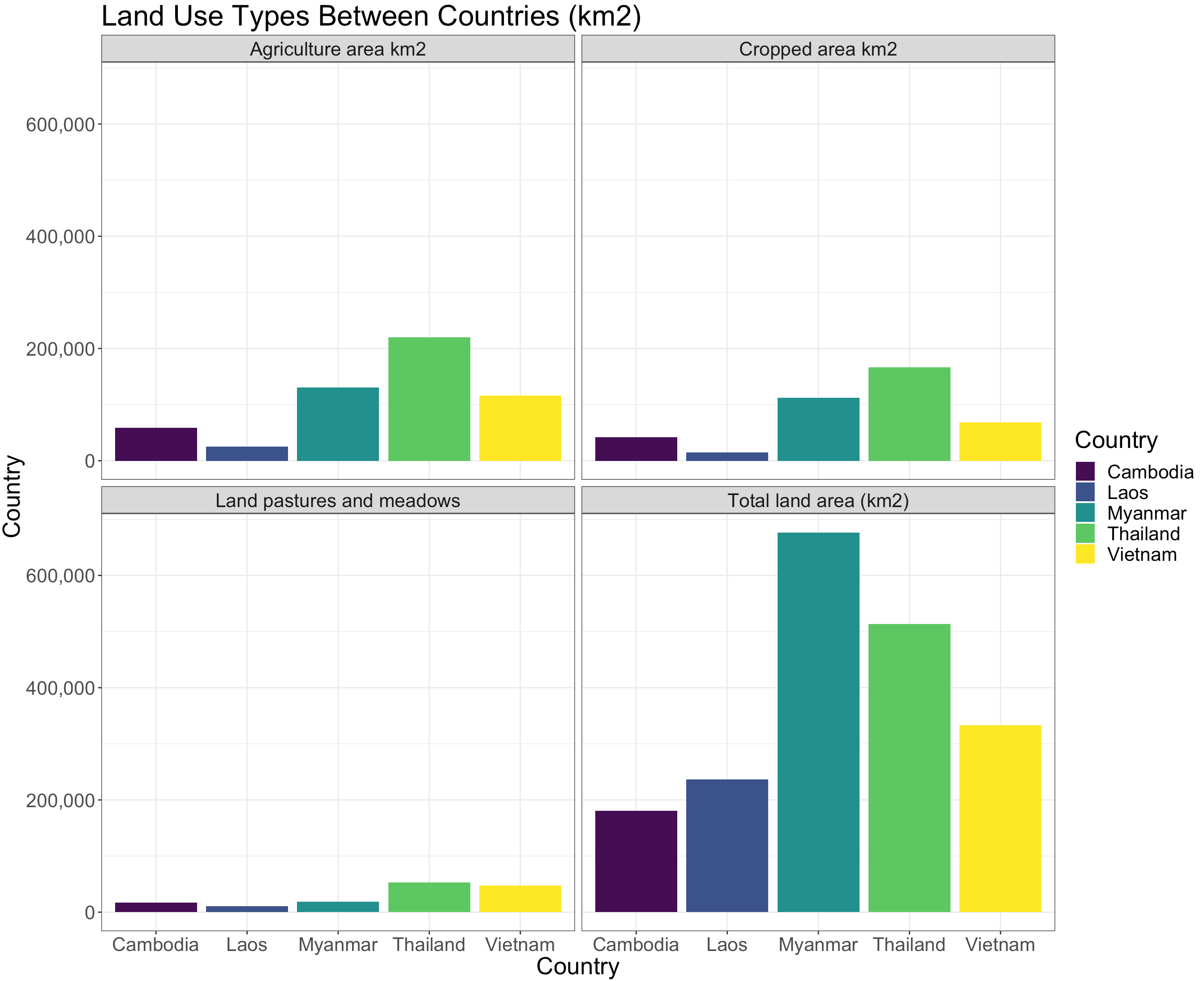 ---  --- #Overall difference between the countries ```r library(formatR) land.indicators.2012.km <- read.csv("land-indicators-2012-km.csv") land.indicators.2012.percent <- read.csv("land-indicators-2012-percent.csv") # Land use by km2 summary(aov(land.indicators.2012.km$Amount ~ land.indicators.2012.km$Country)) ``` ``` ## Df Sum Sq Mean Sq F value Pr(>F) ## land.indicators.2012.km$Country 4 1.068e+11 2.669e+10 0.822 0.531 ## Residuals 15 4.869e+11 3.246e+10 ``` ```r # Land use by percent summary(aov(land.indicators.2012.percent$Amount ~ land.indicators.2012.percent$Country)) ``` ``` ## Df Sum Sq Mean Sq F value Pr(>F) ## land.indicators.2012.percent$Country 4 984.6 246.15 5.756 0.0411 * ## Residuals 5 213.8 42.76 ## --- ## Signif. codes: 0 '***' 0.001 '**' 0.01 '*' 0.05 '.' 0.1 ' ' 1 ``` --- #Where is the difference between countries found? ```r TukeyHSD(aov(land.indicators.2012.percent$Amount ~ land.indicators.2012.percent$Country)) ``` ``` ## Tukey multiple comparisons of means ## 95% family-wise confidence level ## ## Fit: aov(formula = land.indicators.2012.percent$Amount ~ land.indicators.2012.percent$Country) ## ## $`land.indicators.2012.percent$Country` ## diff lwr upr p adj ## Laos-Cambodia -19.424650 -45.656703 6.807403 0.1396226 ## Myanmar-Cambodia -9.995385 -36.227438 16.236668 0.5884065 ## Thailand-Cambodia 9.686365 -16.545688 35.918418 0.6119421 ## Vietnam-Cambodia -0.111285 -26.343338 26.120768 1.0000000 ## Myanmar-Laos 9.429265 -16.802788 35.661318 0.6317063 ## Thailand-Laos 29.111015 2.878962 55.343068 0.0335155 ## Vietnam-Laos 19.313365 -6.918688 45.545418 0.1420955 ## Thailand-Myanmar 19.681750 -6.550303 45.913803 0.1340816 ## Vietnam-Myanmar 9.884100 -16.347953 36.116153 0.5968497 ## Vietnam-Thailand -9.797650 -36.029703 16.434403 0.6034348 ``` --- ## What does this tell us? -- ```r TukeyHSD(aov(land.indicators.2012.percent$Amount ~ land.indicators.2012.percent$Country)) ``` ``` ## Tukey multiple comparisons of means ## 95% family-wise confidence level ## ## Fit: aov(formula = land.indicators.2012.percent$Amount ~ land.indicators.2012.percent$Country) ## ## $`land.indicators.2012.percent$Country` ## diff lwr upr p adj ## Laos-Cambodia -19.424650 -45.656703 6.807403 0.1396226 ## Myanmar-Cambodia -9.995385 -36.227438 16.236668 0.5884065 ## Thailand-Cambodia 9.686365 -16.545688 35.918418 0.6119421 ## Vietnam-Cambodia -0.111285 -26.343338 26.120768 1.0000000 ## Myanmar-Laos 9.429265 -16.802788 35.661318 0.6317063 *## Thailand-Laos 29.111015 2.878962 55.343068 0.0335155 ## Vietnam-Laos 19.313365 -6.918688 45.545418 0.1420955 ## Thailand-Myanmar 19.681750 -6.550303 45.913803 0.1340816 ## Vietnam-Myanmar 9.884100 -16.347953 36.116153 0.5968497 ## Vietnam-Thailand -9.797650 -36.029703 16.434403 0.6034348 ``` --- class: center, inverse, middle ##From this we can interpret that there isn't much of a difference between the countries. There is, however a significant difference between Thailand and Laos, for **what their land is used for**. In general, Laos has used a lot less of their land for agriculture, compared to the other countries but especially compared to Thailand. --- #How did I get to this point? -- ##First, by looking at the data as it was in the `.csv` file.  --- ##Because this is a pretty simple dataset, I decided to do a basic analysis where I try to understand the difference between the countries. I decided to start by **visualizing the data**, using `ggplot2`. (Hopefully you all remember how to use it!) --- ### However, you may have noticed that our data is not easy to use for creating a `ggplot`. I cheated and went to the .csv file to turn my data into a format that could be read by `ggplot`, specifically, where all of the variables are columns. --  --- ### BUT, it wasn't as easy as doing this for the whole dataset. When I looked at the data, the data was represented in different formats, *kilometers squared* and *percent*. So, I had to create two datasets. .pull-left[ ###**km2**  ] .pull-right[ ###**percent**  ] --- class: center, middle ## Hopefully you can see here why we couldn't plot these together. Kilometers squared is on a much larger scale than percent, i.e. 200,000 versus 35. --- To plot this data, I used the following code. Again, this took me some trial and error to get it right for both graphs. ```r require(tidyverse) require(scales) ggplot(land.indicators.2012.km, aes(x = Country, y = Amount, fill = Country)) + geom_bar(stat = "identity") + theme_bw() + scale_fill_viridis_d() + facet_wrap(~Land.Use.Type) + scale_y_continuous(name="Country", labels = comma) + ggtitle("Land Use Types Between Countries (km2)") + theme(text = element_text(size = 20)) ``` ```r ggplot(land.indicators.2012.percent, aes(x = Country, y = Amount, fill = Country)) + geom_bar(stat = "identity") + theme_bw() + scale_fill_viridis_d() + facet_wrap(~Land.Use.Type) + scale_y_continuous(name="Country", labels = comma) + ggtitle("Land Use Types Between Countries (%)") + theme(text = element_text(size = 20)) + scale_x_discrete(limits=c("Thailand","Vietnam","Cambodia", "Myanmar", "Laos")) ``` ---  ---  --- ## As you saw, after visualizing these graphs, I decided to perform an ANOVA on *country* and *amount* (of km2/percent of land used for other purposes), to see whether the country differences seen are significant. ### The ANOVA for percent was significant, so I performed the follow-up test of TUKEY's HSD to determine where the difference was, and found that Thailand and Laos significantly differed in the percent of their land used for agriculture. --- ## And that's it! There are probably all kinds of better and more interesting things that could be done with that data, but that will do for now. --- background-image: url("images/mountain.jpg") class: center, middle, inverse ## Let's take a break --- # Tidying our data with `dplyr` -- class: center, middle ## `dplyr` is a package within the `tidyverse`. It is widely used in R data analysis because it is quick and efficient at cleaning and sorting data. <br><br><br><br><br><br><br><br> #### Disclaimer: I am not very good at using `dplyr` myself! So we will both be learning. --- class: center, middle ## First, we will load the `tidyverse` package (install it if you haven't already). ### We’re going to learn some of the most common dplyr functions: `select()`, `filter()`, `mutate()`, `group_by()`, and `summarise()`. --- # `select()` -- ## As the name implies, this is where we *select* the columns that we want to keep in a data frame. -- ### But first, you'll need to load the data. Do the following: ```r library(nycflights13) flights ``` ``` ## # A tibble: 336,776 x 19 ## year month day dep_time sched_dep_time dep_delay arr_time sched_arr_time ## <int> <int> <int> <int> <int> <dbl> <int> <int> ## 1 2013 1 1 517 515 2 830 819 ## 2 2013 1 1 533 529 4 850 830 ## 3 2013 1 1 542 540 2 923 850 ## 4 2013 1 1 544 545 -1 1004 1022 ## 5 2013 1 1 554 600 -6 812 837 ## 6 2013 1 1 554 558 -4 740 728 ## 7 2013 1 1 555 600 -5 913 854 ## 8 2013 1 1 557 600 -3 709 723 ## 9 2013 1 1 557 600 -3 838 846 ## 10 2013 1 1 558 600 -2 753 745 ## # … with 336,766 more rows, and 11 more variables: arr_delay <dbl>, ## # carrier <chr>, flight <int>, tailnum <chr>, origin <chr>, dest <chr>, ## # air_time <dbl>, distance <dbl>, hour <dbl>, minute <dbl>, time_hour <dttm> ``` #### And take a look at our data using all of the tools I taught you in the first course (`head`, `summary`, and one you may not have used previously: `str`). --- # Using `select()` on your data -- ### The first argument to this function is the data frame (which `dplyr` calls a tibble), and the subsequent arguments are the columns to keep. ### For our data in `flights`, let's use `select` to choose some columns to keep. ```r dplyr::select(flights, year, month, day) ``` ``` ## # A tibble: 336,776 x 3 ## year month day ## <int> <int> <int> ## 1 2013 1 1 ## 2 2013 1 1 ## 3 2013 1 1 ## 4 2013 1 1 ## 5 2013 1 1 ## 6 2013 1 1 ## 7 2013 1 1 ## 8 2013 1 1 ## 9 2013 1 1 ## 10 2013 1 1 ## # … with 336,766 more rows ``` --- # Easy, right? Now let's choose some rows to work with using `filter`. ```r dplyr::filter(flights, month == 1, day == 1) ``` ``` ## # A tibble: 842 x 19 ## year month day dep_time sched_dep_time dep_delay arr_time sched_arr_time ## <int> <int> <int> <int> <int> <dbl> <int> <int> ## 1 2013 1 1 517 515 2 830 819 ## 2 2013 1 1 533 529 4 850 830 ## 3 2013 1 1 542 540 2 923 850 ## 4 2013 1 1 544 545 -1 1004 1022 ## 5 2013 1 1 554 600 -6 812 837 ## 6 2013 1 1 554 558 -4 740 728 ## 7 2013 1 1 555 600 -5 913 854 ## 8 2013 1 1 557 600 -3 709 723 ## 9 2013 1 1 557 600 -3 838 846 ## 10 2013 1 1 558 600 -2 753 745 ## # … with 832 more rows, and 11 more variables: arr_delay <dbl>, carrier <chr>, ## # flight <int>, tailnum <chr>, origin <chr>, dest <chr>, air_time <dbl>, ## # distance <dbl>, hour <dbl>, minute <dbl>, time_hour <dttm> ``` --- ## This lets us filter our data so that it only shows flights on January 1st. -- ### **Remember, if you want to use these commands to create a new dataframe, you need to apply these commands to an object, i.e.: -- ```r *jan_first_flights <- dplyr::filter(flights, month == 1, day == 1) ``` --- # But what if you want to use `select` AND `filter`? --- ## We use something called **pipes**. Pipes look like this ` %>% `. They take the output of one command and put it directly into the next. -- ### Example: ```r flights %>% dplyr::filter(month == 1) %>% dplyr::select(year, month, day, dep_delay) ``` ``` ## # A tibble: 27,004 x 4 ## year month day dep_delay ## <int> <int> <int> <dbl> ## 1 2013 1 1 2 ## 2 2013 1 1 4 ## 3 2013 1 1 2 ## 4 2013 1 1 -1 ## 5 2013 1 1 -6 ## 6 2013 1 1 -4 ## 7 2013 1 1 -5 ## 8 2013 1 1 -3 ## 9 2013 1 1 -3 ## 10 2013 1 1 -2 ## # … with 26,994 more rows ``` --- Class: center, middle ## We perform these commands as part of something called *data carpentry*, i.e. getting your data useable in analysis and visualization. The more you work with data, the more you'll understand what these commands are doing and how they'll help you, down the line. --- # Exercise -- ## Using pipes, subset `flights` to include rows where the year is 2013 and keep only the columns year, month, and dep_delay. ### How many rows are in that tibble? HINT: You can use the nrow() function to find out how many rows are in a tibble. --- # `mutate` ## Frequently you’ll want to create new columns based on the values in existing columns, for example to do unit conversions or find the ratio of values in two columns. For this we’ll use `mutate()` -- ### Let's create a new column of the flight duration. We can do this by using mutate and subtracting `arr_time` (arrival time) from the `dep_time` (departure time). ```r flights %>% mutate(duration = arr_time - dep_time) ``` ``` ## # A tibble: 336,776 x 20 ## year month day dep_time sched_dep_time dep_delay arr_time sched_arr_time ## <int> <int> <int> <int> <int> <dbl> <int> <int> ## 1 2013 1 1 517 515 2 830 819 ## 2 2013 1 1 533 529 4 850 830 ## 3 2013 1 1 542 540 2 923 850 ## 4 2013 1 1 544 545 -1 1004 1022 ## 5 2013 1 1 554 600 -6 812 837 ## 6 2013 1 1 554 558 -4 740 728 ## 7 2013 1 1 555 600 -5 913 854 ## 8 2013 1 1 557 600 -3 709 723 ## 9 2013 1 1 557 600 -3 838 846 ## 10 2013 1 1 558 600 -2 753 745 ## # … with 336,766 more rows, and 12 more variables: arr_delay <dbl>, ## # carrier <chr>, flight <int>, tailnum <chr>, origin <chr>, dest <chr>, ## # air_time <dbl>, distance <dbl>, hour <dbl>, minute <dbl>, time_hour <dttm>, ## # duration <int> ``` --- # Split-apply-combine data analysis and the `summarize()` function -- ## Many data analysis tasks can be approached using the “split-apply-combine” paradigm: 1. Split the data into groups -- 2. Apply some analysis to each group -- 3. And then combine the results. -- `dplyr` makes this very easy through the use of the `group_by()` function, which splits the data into groups. --- ## When the data is grouped in this way `summarize()` can be used to collapse each group into a single-row summary. `summarize()` does this by applying an aggregating or summary function to each group. For example, if we wanted to group by month and find the number of rows of data for each year, we would do: -- ```r flights %>% group_by(month) %>% summarize(n()) ``` ``` ## `summarise()` ungrouping output (override with `.groups` argument) ``` ``` ## # A tibble: 12 x 2 ## month `n()` ## <int> <int> ## 1 1 27004 ## 2 2 24951 ## 3 3 28834 ## 4 4 28330 ## 5 5 28796 ## 6 6 28243 ## 7 7 29425 ## 8 8 29327 ## 9 9 27574 ## 10 10 28889 ## 11 11 27268 ## 12 12 28135 ``` --- ## Of course, that doesn't tell us much that is useful. Let's look at the mean departure delay for each month. -- ```r flights %>% group_by(month) %>% summarize(mean_dep_delay = mean(dep_delay, na.rm = TRUE)) ``` ``` ## `summarise()` ungrouping output (override with `.groups` argument) ``` ``` ## # A tibble: 12 x 2 ## month mean_dep_delay ## <int> <dbl> ## 1 1 10.0 ## 2 2 10.8 ## 3 3 13.2 ## 4 4 13.9 ## 5 5 13.0 ## 6 6 20.8 ## 7 7 21.7 ## 8 8 12.6 ## 9 9 6.72 ## 10 10 6.24 ## 11 11 5.44 ## 12 12 16.6 ``` --- ### The `na.rm` here is where we tell R to ignore any missing data which usually is shown as "NA". If we don't use this command and we have missing data, R will return an error. --- ## You can also group by multiple columns, which is very handy! -- ```r flights %>% group_by(carrier, month) %>% summarize(mean_dep_delay = mean(dep_delay, na.rm = TRUE)) ``` ``` ## `summarise()` regrouping output by 'carrier' (override with `.groups` argument) ``` ``` ## # A tibble: 185 x 3 ## # Groups: carrier [16] ## carrier month mean_dep_delay ## <chr> <int> <dbl> ## 1 9E 1 16.9 ## 2 9E 2 16.5 ## 3 9E 3 13.4 ## 4 9E 4 13.6 ## 5 9E 5 22.7 ## 6 9E 6 29.0 ## 7 9E 7 31.4 ## 8 9E 8 17.3 ## 9 9E 9 7.75 ## 10 9E 10 9.33 ## # … with 175 more rows ``` --- ## You can also use summarize on multiple variables (columns, for our flights data). For our example, let's look at the mean delay as well as the minimum value for departure time: -- ```r flights %>% group_by(carrier, month) %>% summarize(mean_dep_delay = mean(dep_delay, na.rm = TRUE), min_generation = min(dep_time, na.rm = TRUE)) ``` ``` ## `summarise()` regrouping output by 'carrier' (override with `.groups` argument) ``` ``` ## # A tibble: 185 x 4 ## # Groups: carrier [16] ## carrier month mean_dep_delay min_generation ## <chr> <int> <dbl> <int> ## 1 9E 1 16.9 15 ## 2 9E 2 16.5 555 ## 3 9E 3 13.4 14 ## 4 9E 4 13.6 15 ## 5 9E 5 22.7 33 ## 6 9E 6 29.0 7 ## 7 9E 7 31.4 13 ## 8 9E 8 17.3 651 ## 9 9E 9 7.75 3 ## 10 9E 10 9.33 636 ## # … with 175 more rows ``` --- # Long to wide and wide to long -- ## Our flights data is currently in "long" format, which is usually (but not always!!) how you are going to want your data to be, for the kinds of data analyses you'll be doing. Sometimes, you want to turn your data wide. --- ## To do this, we can make our data wide and compare carriers and their departure delays. This is again easy to do with `dplyr`, using the `spread` function. -- ```r library(nycflights13) flights_wide <- flights %>% tidyr::spread(carrier, dep_delay) flights_wide ``` ``` ## # A tibble: 336,776 x 33 ## year month day dep_time sched_dep_time arr_time sched_arr_time arr_delay ## <int> <int> <int> <int> <int> <int> <int> <dbl> ## 1 2013 1 1 517 515 830 819 11 ## 2 2013 1 1 533 529 850 830 20 ## 3 2013 1 1 542 540 923 850 33 ## 4 2013 1 1 544 545 1004 1022 -18 ## 5 2013 1 1 554 600 812 837 -25 ## 6 2013 1 1 554 558 740 728 12 ## 7 2013 1 1 555 600 913 854 19 ## 8 2013 1 1 557 600 709 723 -14 ## 9 2013 1 1 557 600 838 846 -8 ## 10 2013 1 1 558 600 753 745 8 ## # … with 336,766 more rows, and 25 more variables: flight <int>, tailnum <chr>, ## # origin <chr>, dest <chr>, air_time <dbl>, distance <dbl>, hour <dbl>, ## # minute <dbl>, time_hour <dttm>, `9E` <dbl>, AA <dbl>, AS <dbl>, B6 <dbl>, ## # DL <dbl>, EV <dbl>, F9 <dbl>, FL <dbl>, HA <dbl>, MQ <dbl>, OO <dbl>, ## # UA <dbl>, US <dbl>, VX <dbl>, WN <dbl>, YV <dbl> ``` --- ## What is happening with this command? -- ### `spread` requires you tell it the name of the column which contains values that will be the column names in your new data set - a so called “key” column. You also tell it which column contains the relevant numbers - the “values” column. -- ### In our example here, we see that there are quitea lot of NAs, so this is not a sensible way to organize our data. --- # As I told you a few minutes ago, you guys will usually be working with "long" data. So, you will want to know how to transform your "wide" data into this format. -- ## For this, you will use the `gather` function. -- ### In this case you specify what you want the name of the new key column to be, what you want the name of the new values column to be, and then you can either specify which columns are to be gathered up (which can be tedious if there are a lot or they are spread) or you can specify which columns you want to exclude. -- I will show you an example where we *exclude* a column. --- ```r # First we create a dataset called stocks stocks <- tibble( time = as.Date('2009-01-01') + 0:9, X = rnorm(10, 0, 1), Y = rnorm(10, 0, 2), Z = rnorm(10, 0, 4) ) #Then we use gather to change the wide data into long format stocks %>% gather("stock", "price", -time) ``` ``` ## # A tibble: 30 x 3 ## time stock price ## <date> <chr> <dbl> ## 1 2009-01-01 X 1.06 ## 2 2009-01-02 X -0.686 ## 3 2009-01-03 X 0.276 ## 4 2009-01-04 X 0.730 ## 5 2009-01-05 X -0.624 ## 6 2009-01-06 X 0.136 ## 7 2009-01-07 X -1.24 ## 8 2009-01-08 X 1.06 ## 9 2009-01-09 X 0.258 ## 10 2009-01-10 X -0.00981 ## # … with 20 more rows ``` --- class: center, middle # And that's it! You now know the basics of data carpentry with `dplyr`. -- ## Of course, R being R there is always more to learn, so be sure to check out the "Helpful R Sites" document to see examples of more tutorials. --- class: center, middle, inverse # Acknowledgements ### Grateful thanks to everyone on Twitter and especially Aleeza Gerstein at the University of Manitoba for kindly sharing her materials.